Wave Shaping

Integrators

The integrator (RC or RL) is used as a waveshaping network e.g. in communications, radar systems, and computers. A square wave is frequently applied to the integrators. The harmonic content of the square wave is made up of odd multiples of the fundamental frequency. Therefore significant harmonics (those that have an effect on the circuit) as high as 50 or 60 times the fundamental frequency will be present in the wave.

RC Integrators

The capacitor will offer a reactance (X_C) of a different magnitude to each of the harmonics

This means that the voltage drop across the capacitor for each harmonic frequency present will not be the same. To low frequencies, the capacitor will offer a large opposition, providing a large voltage drop across the capacitor. To high frequencies, the reactance of the capacitor will be extremely small, causing a small voltage drop across the capacitor. This is no different than is the case for low- and high-pass filters (discriminators) presented later. If the voltage component of the harmonic is not developed across the reactance of the capacitor, it will be developed across the resistor, if we observe Kirchhoff's voltage law. The harmonic amplitude and phase relationship across the capacitor is not the same as that of the original frequency input; therefore, a perfect square wave will not be produced across the capacitor. You should remember that the reactance offered to each harmonic frequency will cause a change in both the amplitude and phase of each of the individual harmonic frequencies with respect to the current reference. The amount of phase and amplitude change taking place across the capacitor depends on the X_C of the capacitor. The value of the resistance offered by the resistor must also be considered here; it is part of the ratio of the voltage development across the network.

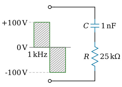
The circuit in the figure above will help show the relationships of R and X_C more clearly. The square wave applied to the circuit is 100 volts peak at a frequency of 1 kilohertz. The odd harmonics will be 3 kilohertz, 5 kilohertz, 7 kilohertz, etc. The table below shows the values of X_C and R offered to several harmonics and indicates the approximate value of the cutoff frequency (X_C = R). The table clearly shows that the cutoff frequency lies between the fifth and seventh harmonics. Between these two values, the capacitive reactance will equal the resistance. Therefore, for all harmonic frequencies above the fifth, the majority of the output voltage will not be developed across the output capacitor. Rather, most of the output will be developed across R. The absence of the higher order harmonics will cause the leading edge of the waveform developed across the capacitor to be rounded. An example of this effect is shown in the figure below. If the value of the capacitance is increased, the reactances to each harmonic frequency will be further decreased. This means that even fewer harmonics will be developed across the capacitor.

Harmonic	XC (kΩ)	R (kΩ)
Fundamental	159	25
3rd	53	25
5th	31.8	25
7th	22.7	25
9th	17.7	25
11th	14.5	25

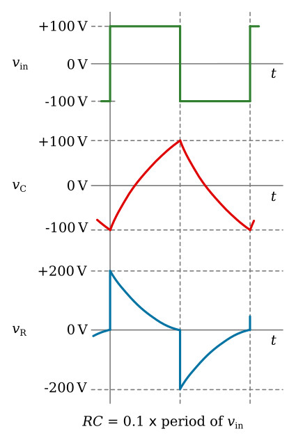
The harmonics not effectively developed across the capacitor must be developed across the resistor to satisfy Kirchhoff's voltage law. Note the pattern of the voltage waveforms across the resistor and capacitor. If the waveforms across both the resistor and the capacitor were added graphically, the resultant would be an exact duplication of the input square wave.

When the capacitance is increased sufficiently, full integration of the input signal takes place in the output across the capacitor. An example of complete integration is shown in the figure below (waveform v_C). This effect can be caused by significantly decreasing the value of capacitive reactance. The same effect would take place by increasing the value of the resistance. Integration takes place in an RC circuit when the output is taken across the capacitor.

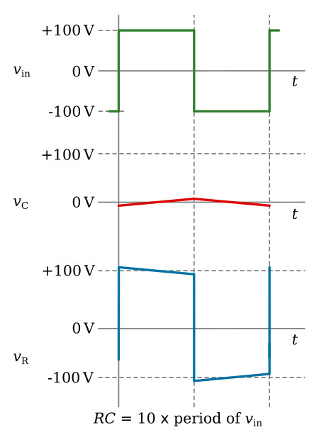
The amount of integration is dependent upon the values of R and C. The amount of integration may also be dependent upon the time constant of the circuit. The time constant of the circuit should be at least 10 times greater than the time duration of the input pulse for integration to occur. The value of 10 is only an approximation. When the time constant of the circuit is 10 or more times the value of the duration of the input pulse, the circuit is said to possess a long time constant. When the time constant is long, the capacitor does not have the ability to charge instantly to the value of the applied voltage. Therefore, the result is the long, sloping, integrated waveform.

RL Integrators

The RL circuit may also be used as an integrating circuit. An integrated waveform may be obtained from the series RL circuit by taking the output across the resistor. The characteristics of the inductor are such that at the first instant of time in which voltage is applied, current flow through the inductor is minimum and the voltage developed across it is maximum. Therefore, the value of the voltage drop across the series resistor at that first instant must be 0 volts because there is no current flow through it. As time passes, current begins to flow through the circuit and voltage develops across the resistor. Since the circuit has a long time constant, the voltage across the resistor does not respond to the rapid changes in voltage of the input square wave. Therefore, the conditions for integration in an RL circuit are a long time constant with the output taken across the resistor. These conditions are shown in the figure below.

Integrator Waveform Analysis

If either an RC or RL circuit has a time constant 10 times greater than the duration of the input pulse, the circuits are capable of integration. Let's compute and graph the actual waveform that would result from a long time constant (10 times the pulse duration), a short time constant (1/10 of the pulse duration), and a medium time constant (that time constant between the long and the short). To accurately plot values for the capacitor output voltage, we will use the Universal Time Constant Chart shown in the figure below.

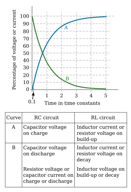
You already know that capacitor charge follows the shape of the curve shown in the figure above. This curve may be used to determine the amount of voltage across either component in the series RC circuit. As long as the time constant or a fractional part of the time constant is known, the voltage across either component may be determined.

Short Time-Constant Integrator

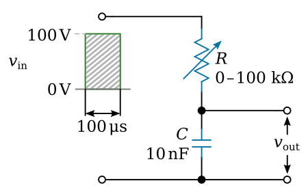
In the figure above, a 100-microsecond pulse at an amplitude of 100 volts is applied to the circuit. The circuit is composed of the 0.01 μF capacitor and the variable resistor R. The square wave applied is a pure square wave. The resistance of the variable resistor is set at a value of 1,000 ohms. The time constant of the circuit is given by the equation:

Substituting values:

Since the time constant of the circuit is 10 microseconds and the pulse duration is 100 microseconds, the time constant is short (1/10 of the pulse duration). The capacitor is charged exponentially through the resistor. In 5 time constants, the capacitor will be, for all practical purposes, completely charged. At the first time constant, the capacitor is charged to 63.2 volts, at the second 86.5 volts, at the third 95 volts, at the fourth 98 volts, and finally at the end of the fifth time constant (50 microseconds), the capacitor is almost fully charged. This is shown in the figure below.

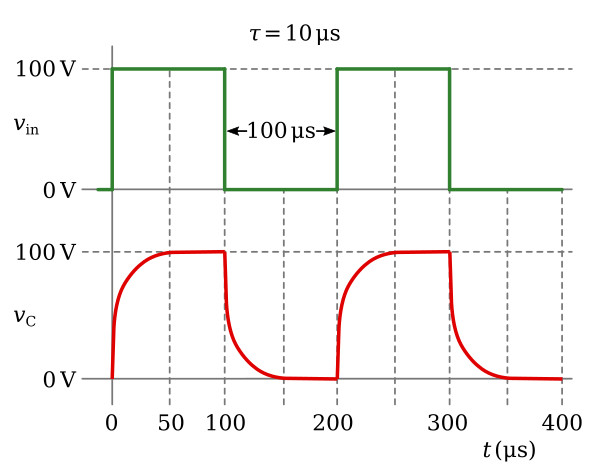
Notice that the leading edge of the square wave taken across the capacitor is rounded. If the time constant were made extremely short, the rounded edge would become square.

Medium Time-Constant Integrator

The time constant, in the figure above can be changed by increasing the value of the variable resistor to 10,000 ohms. The time constant will then be equal to 100 microseconds.

This time constant is known as a medium time constant. Its value lies between the extreme ranges of the short and long time constants. In this case, its value happens to be exactly equal to the duration of the input pulse, 100 microseconds. The output waveform, after several time constants, is shown in the figure below. The long, sloping rise and fall of voltage is caused by the inability of the capacitor to charge and discharge rapidly through the 10,000-ohm series resistance.

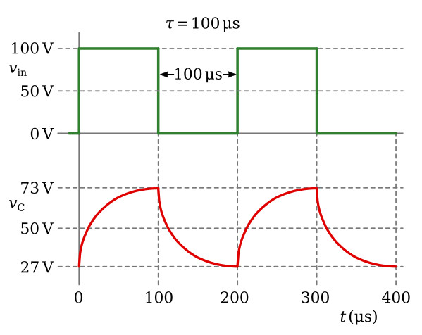
At the first instant of time, 100 volts is applied to the medium time-constant circuit. In this circuit, 1τ is exactly equal to the duration of the input pulse. After 1τ the capacitor has charged to 63.2 percent of the input voltage (100 volts). Therefore, at the end of 1τ (100 microseconds), the voltage across the capacitor is equal to 63.2 volts. However, as soon as 100 microseconds has elapsed, and the initial charge on the capacitor has risen to 63.2 volts, the input voltage suddenly drops to 0. It remains there for 100 microseconds. The capacitor will now discharge for 100 microseconds. Since the discharge time is 100 microseconds (1τ), the capacitor will discharge 63.2 percent of its total 63.2-volt charge, a value of 23.3 volts. During the next 100 microseconds, the input voltage will increase from 0 to 100 volts instantaneously. The capacitor will again charge for 100 microseconds (1τ). The voltage available for this charge is the difference between the voltage applied and the charge on the capacitor (100 - 23.3 volts), or 76.7 volts. Since the capacitor will only be able to charge for 1τ, it will charge to 63.2 percent of the 76.7 volts, or 48.4 volts. The total charge on the capacitor at the end of 300 microseconds will be 23.3 + 48.4 volts, or 71.7 volts.

Notice that the capacitor voltage at the end of 300 microseconds is greater than the capacitor voltage at the end of 100 microseconds. The voltage at the end of 100 microseconds is 63.2 volts, and the capacitor voltage at the end of 300 microseconds is 71.7 volts, an increase of 8.5 volts.

The output waveform in this graph (v_C) is the waveform that will be produced after many cycles of input signal to the integrator. The capacitor will charge and discharge in a step-by-step manner until it finally charges and discharges above and below a 50-volt level. The 50-volt level is controlled by the maximum amplitude of the symmetrical input pulse, the average value of which is 50 volts.

Long Time-Constant Integrator

If the resistance in the RC integrator is increased to 100,000 ohms, the time constant of the circuit will be 1,000 microseconds. This time constant is 10 times the pulse duration of the input pulse. It is, therefore, a long time-constant circuit.

The shape of the output waveform across the capacitor is shown in the figure below. The shape of the output waveform is characterized by a long, sloping rise and fall of capacitor voltage.

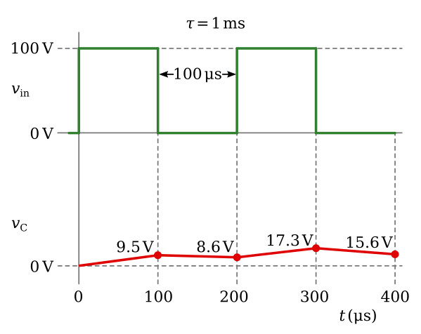
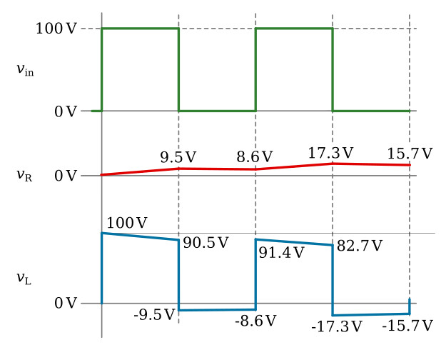
At the first instant of time, 100 volts is applied to the long time-constant circuit. The value of charge on the capacitor at the end of the first 100 microseconds of the input signal can be found by using the Universal Time Constant Chart. Assume that a line is projected up from the point on the base line corresponding to 0.1τ. The line will intersect the curve at a point that is the percentage of voltage across the capacitor at the end of the first 100 microseconds. Since the applied voltage is 100 volts, the charge on the capacitor at the end of the first 100 microseconds will be approximately 9.5 volts. At the end of the first 100 microseconds, the input signal will fall suddenly to 0 and the capacitor will begin to discharge. It will be able to discharge for 100 microseconds. Therefore, the capacitor will discharge 9.5 percent of its accumulated 9.5 volts (0.095 × 9.5 = 0.90 volt). The discharge of the 0.90 volt will result in a remaining charge on the capacitor of 8.6 volts. At the end of 200 microseconds, the input signal will again suddenly rise to a value of 100 volts. The capacitor will be able to charge to 9.5 percent of the difference (100 - 8.6 = 91.4 volts). This may also be figured as a value of 8.7 volts plus the initial 8.6 volts. This results in a total charge on the capacitor (at the end of the first 300 microseconds) of 8.7 + 8.6 = 17.3 volts.

Notice that the capacitor voltage at the end of the first 300 microseconds is greater than the capacitor voltage at the end of the first 100 microseconds. The voltage at the end of the first 100 microseconds is 9.5 volts; the capacitor voltage at the end of the first 300 microseconds is 17.3 volts, an increase of 7.8 volts.

The capacitor charges and discharges in this step-by-step manner until, finally, the capacitor charges and discharges above and below a 50-volt level. The 50-volt level is controlled by the maximum amplitude of the square-wave input pulse, the average value of which is 50 volts.