Filters

Frequency and Impedance Scaling

For purposes of standardization and simplification, a filter can be initially designed to provide some convenient cutoff frequency such as f = 1 Hz (or, more usually, ω = 1 rad/s) and to incorporate convenient impedance levels such as one ohm, even though the final result might yield impractical component values. The filter is then redesigned to the desired frequency and to practical impedance levels by frequency and impedance scaling.

The simple low-pass filter shown in the figure below (view A) has a cutoff frequency of ω_C = 1/(RC) = 1 rad/s. It is called a normalized filter because its cutoff frequency is 1 rad/s and because its component values are unity (ohm-farad). The normalized amplitude response is shown in view A of the figure.

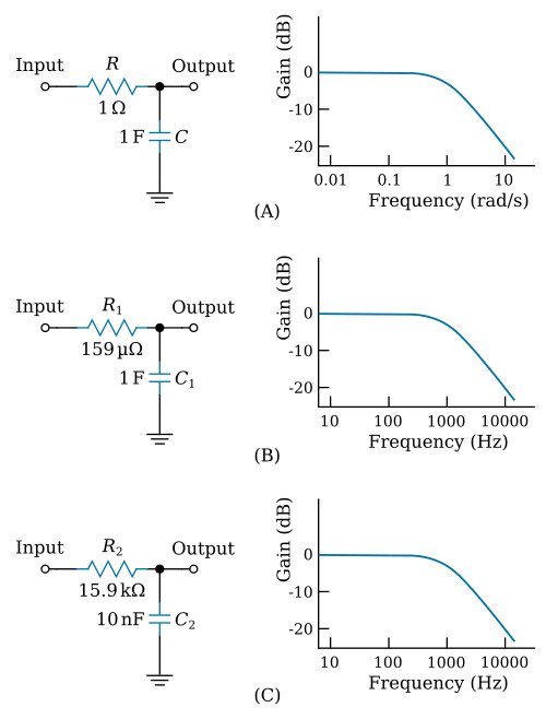
Suppose a filter is required that can be constructed from practical components and that has the same amplitude response curve shape as in the figure above (view A), but with a cutoff frequency of 1000 Hz. Since ω_C is proportional to the reciprocal of the RC product, the frequency can be increased by reducing R, C, or both. The multiplying factor is the ratio of the normalized frequency f = ω/2π = 1/2π Hz, to the desired frequency of 1000 Hz. Note that frequencies should be either in radians per second or, as chosen in this case, cycles per second (Hz). Further, let it be decided to reduce R and leave C at one farad. The new resistance will be

The figure above (view B) shows the design of the filter at this stage. Three observations can be made at this point: First, the filter has been adjusted to the correct cutoff frequency of 1000 Hz. Second, the shape of the amplitude response curve has not been changed by frequency scaling, so, theoretically, the design is complete. Third, the design involves completely impractical component values of R₁ = 0.000159 Ω and C₁ = 1 F. Fortunately, the frequency is proportional to the reciprocal of the product of R₁ and C₁; thus if one is increased and the other decreased by the same amount, the frequency will remain unchanged. Consequently, a more practical component selection can be obtained by converting the initial C₁ value of 1 F to 10 nF by dividing by 10⁸. To keep the cutoff frequency at 1000 Hz, R₁ must be multiplied by 10⁸ to give 15,900 Ω. The final circuit and its response are shown in the figure above (view C).

Note that the amplitude responses indicated in views B and C of the figure above are identical in shape and cutoff frequency, which illustrates that impedance scaling does not change the response curve in any way. The procedures used to scale frequency and impedance are general and can be applied to various filters. The rules are summarized in the table below.

Frequency scaling	Given a filter that has a cutoff frequency of fC, change to a new cutoff frequency fn as follows: Either multiply all resistor values by fC/fn or multiply all capacitor values by fC/fn
Impedance scaling	Multiply all resistors by k and divide all capacitors by k, where k is any suitable constant that will bring the impedances to the desired levels. Note that k can be greater or less than unity, so that R's can be increased and C's decreased or vice versa as desired. Note that the cutoff frequency fC is not altered by impedance scaling.