


Home > Textbooks > Basic Electronics > Filters > Transfer Functions >
Filters
Transfer Functions
The design of filters involves a detailed consideration of input/output relationships because a filter may be required to pass or attenuate input signals so that the output amplitude-versus-frequency curve has some desired shape. The purpose of this section is to demonstrate how the equations that describe output-versus-input relationships of filters can be written directly in a mathematical form called a transfer function.
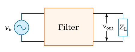
When a voltage is applied to the filter of figure below, the transfer function is H(s) and it is equivalent to (vout/vin) (s), s being in general a complex mathematical operator having both real and imaginary parts (Laplace operator); in this text, however, s will be equated to its steady-state sinusoidal equivalent (jω). The magnitude of the complex transfer function |H(jω)| is then referred to as amplitude response, while the phase of the complex transfer function is called phase response.
The transfer function can be expressed as the ratio of two polynomials, N(s) in the numerator and D(s) in the denominator, such as

The roots of the polynomial in the denominator D(s) are referred to as poles, and the roots of N(s), which are located in the numerator, are referred to as zeros. The order of the filter is the largest exponent of s in the polynomials.
It is possible to study quite generalized expressions for transfer functions, but in order to understand certain essential points, attention will be focused on three specific transfer functions: those for low-pass, high-pass, and band pass filters of the second order. The term "second order" refers to the fact that the transfer equations involve terms no higher than s2. Second-order transfer functions describe 2-pole filters; third-order functions involve s3 and describe 3-pole filters, and so on. Second-order transfer functions are a useful starting point in the study of filters because they are foundations upon which more complex filters can be built.
Typical second-order transfer functions for low-pass, high-pass, and bandpass filters are:

Note that all three transfer functions have the same denominator and that the numerators have increasing powers of s. That the equations do represent low-pass, high-pass, and bandpass filters can be seen by noting that s is proportional to frequency and by studying the behavior of the equations at such points as ω = 0 and ω = ∞. For example, putting ω = 0 into the above equation for low-pass filter K/(s2+bs+a) gives H = K/a, while ω = ∞ gives H = 0, which indicates that this equation describes a filter that passes DC with a gain of K/a and attenuates infinite at high frequencies; in other words, it describes a low-pass filter.
The numerator and the denominator of the above equation for bandpass filter Ks/(s2+bs+a) can be divided by s and then s can be replaced with jω to give

At ω = 0 and ω = ∞, the above equation reduces to zero; when ω = a/ω or ω2 = a, the H is equal to K/b, which indicates that this equation describes a filter that attenuates low and high frequencies and passes midband frequencies; in other words, the equation describes a bandpass filter.
The numerator and denominator of the above equation for high-pass filter Ks2/(s2+bs+a) can be divided by s2 and s can be replaced with jω to give

This equation reduces to 0 at ω = 0 and to K at ω = ∞, indicating that the equation describes a filter that passes high frequencies and attenuates low frequencies; in other words, the equation describes a high-pass filter.
Although the above equation K/(s2+bs+a) describes a low-pass filter, there are many different types of low-pass filters; for example, the next section contains information about Butterworth, Chebyshev, and Bessel low-pass filters. The type of filter, that is, the shape of its response curve, is determined by the constants a and b in the equation for low-pass filter; the constant K is a multiplier that affects the filter gain. Constants a and b in the above equations for bandpass and high-pass filters also determine the type of filter and K is again a multiplying factor affecting the gain.
There are available tables listing constants such as a and b for various types of filters. (K is a scaling factor chosen by the designer to give a specific gain.) Typically, a and b are given as coefficients in polynomial functions for various types of filters.


